GSP866

Overview

This lab introduces you to BigQuery GIS. BigQuery GIS allows you to easily analyze and visualize geospatial data in BigQuery.

This is an introductory lab that is intended for data analysts. A data analyst uses BigQuery standard SQL to analyze data trends that inform business strategy and operations. This includes using BigQuery ML to train ML models, to evaluate ML models, and to do predictive analytics.

What you'll do

In this lab you:

• Use a BigQuery GIS function to convert latitude and longitude columns into geographical points
• Run a query that finds all the Citi Bike stations with more than 30 bikes available for rental
• Visualize your results in BigQuery Geo Viz

Setup and requirements

Before you click the Start Lab button

Read these instructions. Labs are timed and you cannot pause them. The timer, which starts when you click Start Lab, shows how long Google Cloud resources will be made available to you.

This hands-on lab lets you do the lab activities yourself in a real cloud environment, not in a simulation or demo environment. It does so by giving you new, temporary credentials that you use to sign in and access Google Cloud for the duration of the lab.

To complete this lab, you need:

• Access to a standard internet browser (Chrome browser recommended).

Note: Use an Incognito or private browser window to run this lab. This prevents any conflicts between your personal account and the Student account, which may cause extra charges incurred to your personal account.

• Time to complete the lab---remember, once you start, you cannot pause a lab.

Note: If you already have your own personal Google Cloud account or project, do not use it for this lab to avoid extra charges to your account.

Task 1. Explore the NYC Citi Bike Trips dataset

This lab uses a dataset available through the Google Cloud Public Dataset Program. A public dataset is any dataset that is stored in BigQuery and made available to the general public. The public datasets are datasets that BigQuery hosts for you to access and integrate into your applications. Google pays for the storage of these datasets and provides public access to the data via a project. You pay only for the queries that you perform on the data (the first 1 TB per month is free, subject to query pricing details).

Citi Bike is the nation's largest bike share program, with 10,000 bikes and 600 stations across Manhattan, Brooklyn, Queens, and Jersey City. The dataset we use here includes daily Citi Bike trips since Citi Bike launched in September 2013. The data has been processed by Citi Bike to remove trips that are taken by staff to service and inspect the system, as well as any trips below 60 seconds in length, which are considered false starts.

Sample a few rows of data

You can start exploring this data in the BigQuery console by viewing the details of the citibike_stations table.

1. Open the BigQuery web UI in Google Cloud Console, select Navigation menu () > BigQuery.

The Welcome to BigQuery in the Cloud Console message box opens. This message box provides a link to the quickstart guide and lists UI updates.

2. Click Done.

3. Query a few rows from bigquery-public-data.new_york_citibike.citibike_stations to get an understanding of the data stored inside the table. Add the following query into the Query editor text area:

SELECT * FROM `bigquery-public-data.new_york_citibike.citibike_stations` LIMIT 10

4. Click the Run button to execute your query.

Three columns in this table are relevant to this lab:

• longitude: The longitude of a station. The values are valid WGS 84 longitudes in decimal degrees format.
• latitude: The latitude of a station. The values are valid WGS 84 latitudes in decimal degrees format.
• num_bikes_available: The number of bikes available for rental.

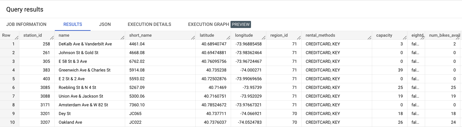
Find the stations with more than 30 bikes available

Next, run a standard SQL query that finds all the Citi Bike stations in New York City with more than 30 bikes available to rent.

1. The following standard SQL query is used to find the Citi Bike stations with more than 30 bikes. Add this query into the Query editor text area:

-- Finds Citi Bike stations with > 30 bikes SELECT ST_GeogPoint(longitude, latitude) AS WKT, num_bikes_available FROM `bigquery-public-data.new_york.citibike_stations` WHERE num_bikes_available > 30

The query clauses do the following:

• SELECT ST_GeogPoint(longitude, latitude) AS WKT, num_bikes_available The SELECT clause selects the num_bikes_available column and uses the ST_GeogPoint function to convert the values in the latitude and longitude columns to GEOGRAPHY types (points).

• FROM bigquery-public-data.new_york.citibike_stations The FROM clause specifies the table being queried: citibike_stations.

• WHERE num_bikes_available > 30 The WHERE clause filters the values in the num_bikes_available column to just those stations with more than 30 bikes.

2. Click the Run button to execute the query.

The query takes a moment to complete. After the query runs, your results appear in the Query results pane.

Test completed task

Click Check my progress to verify your performed task. If you have completed the task successfully you will be granted with an assessment score.

Find the stations with more than 30 bikes available

Visualize the query results in Geo Viz

Next, visualize your results using BigQuery Geo Viz — A web tool for visualization of geospatial data in BigQuery using Google Maps APIs.

1. Open the Geo Viz web tool in a new tab on your browser.

2. Under Query click Authorize.

3. In the pop-up window click your QwikLabs username to authenticate.

4. Click Allow on the next page of the dialog to give Geo Viz access to your BigQuery data.

Note: If you are unable to perform the task in an Incognito window then please perform this step in a normal window.

5. After you authenticate and grant access, the next step is to run a query in Geo Viz. For step one, enter your Project ID in the Project ID field.
6. In the query window, enter the following standard SQL query:

-- Finds Citi Bike stations with > 30 bikes SELECT ST_GeogPoint(longitude, latitude) AS WKT, num_bikes_available FROM `bigquery-public-data.new_york.citibike_stations` WHERE num_bikes_available > 30

7. For Processing Location, choose United States (US). When you query a public dataset, choose United States (US) as the processing location because the public datasets are stored in the US.

8. Click the Run button.

9. View the output of your query by clicking on Show results. Check that the query results are consistent with your expectations.

10. For Geometry column, choose WKT if it's not already selected. This plots the points corresponding to the bike stations on your map.

Test completed task

Click Check my progress to verify your performed task. If you have completed the task successfully you will be granted with an assessment score.

Visualize the query results in Geo Viz

Format your visualization

The Style section provides a list of visual styles for customization. Certain properties apply only to certain types of data. For example, circleRadius affects only points.

Supported style properties include:

• fillColor: The fill color of a polygon or point. For example, "linear" or "interval" functions can be used to map numeric values to a color gradient.
• fillOpacity: The fill opacity of a polygon or point. Values must be in the range zero — one where 0 = transparent and 1 = opaque.
• strokeColor: The stroke or outline color of a polygon or line.
• strokeOpacity: The stroke or outline opacity of polygon or line. Values must be in the range zero — one where 0 = transparent and 1 = opaque.
• strokeWeight: The stroke or outline width in pixels of a polygon or line.
• circleRadius: The radius of the circle representing a point in pixels. For example, a "linear" function can be used to map numeric values to point sizes to create a scatterplot style.

Each style may be given either a global value (applied to every result) or a data-driven value (applied in different ways depending on data in each result row). For data-driven values, the following are used to determine the result:

• function: A function used to compute a style value from a field's values.
• identity: The data value of each field is used as the styling value.
• categorical: The data values of each field listed in the domain are mapped one to one with corresponding styles in the range.
• interval: Data values of each field are rounded down to the nearest value in the domain and are then styled with the corresponding style in the range.
• linear: Data values of each field are interpolated linearly across values in the domain and are then styled with a blend of the corresponding styles in the range.
• field: The specified field in the data is used as the input to the styling function.
• domain: An ordered list of sample input values from a field. Sample inputs (domain) are paired with sample outputs (range) based on the given function and are used to infer style values for all inputs (even those not listed in the domain). Values in the domain must have the same type (text, number, and so on) as the values of the field you are visualizing.
• range: A list of sample output values for the style rule. Values in the range must have the same type (color or number) as the style property you are controlling. For example, the range of the fillColor property should contain only colors.

To format your map:

1. Click the Add styles button on the left-side menu.
2. Change the color of your points. Click fillColor.
3. In the Value field, enter #0000FF, the HTML color code for blue.
4. Examine your map. If you click one of your points, the value is displayed.
5. Click fillOpacity and in the Value field enter .5. Examine your map. The fill color of the points is now semi-transparent.
6. Change the size of the points based on the number of bikes available. Click circleRadius.
7. In the circleRadius panel:

• Enable Data driven.
• For Function, choose linear.
• For Field, choose num_bikes_available.
• For Domain, enter 30 in the first box and 60 in the second.
• For Range, enter 20 in the first box and 450 in the second.

8. Click Apply Style.

9. Examine your map. The radius of each circle now corresponds to the number of bikes available at that location.

Depending on the resolution of your screen you might need to adjust the Range values to make the dynamic data point circle scaling more obvious.

10. Close Geo Viz.

Congratulations

You have used the BigQuery GIS function to analyze a public dataset and visualized your results with BigQuery Geo Viz.

Google Cloud training and certification

...helps you make the most of Google Cloud technologies. Our classes include technical skills and best practices to help you get up to speed quickly and continue your learning journey. We offer fundamental to advanced level training, with on-demand, live, and virtual options to suit your busy schedule. Certifications help you validate and prove your skill and expertise in Google Cloud technologies.

Manual Last Updated: October 03, 2023

Lab Last Tested: October 06, 2023

Copyright 2024 Google LLC All rights reserved. Google and the Google logo are trademarks of Google LLC. All other company and product names may be trademarks of the respective companies with which they are associated.